dvd km

This project was originally for my Math 221 class, Advanced Matrix Computations. Afterwards, I expanded on this work and presented at Yale’s YURC 2026 conference. To read a full version of my report, see here.

A brief background on FNOs

Fourier Neural Operators (FNO) are learned linear integral operators that map input functions to solution functions of PDEs. They replace Galerkin/finite-difference matrices with a trainable spectral convolution using FFTs.

Most translation-invariant PDE solution operators can be represented as integral operators of the form

$$(\mathcal{K} u)(x) = \int_{\Omega} K(x-y)u(y) \, dy$$

where this operator’s kernel $K(x-y)$ encodes Green’s function-like behavior. This operator is diagonalized by the Fourier convolution theorem in the frequency domain:

$$\widehat{\mathcal{K} u}(k) = \hat{K}(k) \hat{u}(k)$$

The Fourier modes $k$ independently evolve through multiplication with complex gain $\hat{K}(k)$. Knowing this, we are able to construct the Fourier Neural Operator with

$$v_{\ell+1}(x) = \sigma \left( \mathcal{F}^{-1} ( M_\ell(k) \mathcal{F}[v_\ell](k) ) + W_\ell v_\ell(x) + b_\ell \right)$$

where:

• $v_\ell(x) \in \mathbb{R}^{d_v}$ denotes the feature field at layer $\ell$
• $\mathcal{F}, \mathcal{F}^{-1}$ = Fourier and inverse Fourier transforms
• $M_\ell(k) \in \mathbb{C}^{w_{\ell+1} \times w_\ell}$ = trainable multiplier matrix per mode $k$
• $W_\ell$ = pointwise linear (1×1 convolution)
• $b_\ell$ = bias
• $\sigma$ = nonlinearity (e.g., ReLU, GELU)

Each FNO layer applies a global Fourier convolution, followed by a local nonlinear map and nonlinearity.

Application Significance

FNOs learn solution operators for families of PDEs, which reduces numerical solves and computation time with quick inference. In practice, FNOs are used in climate/ocean modeling, forecasting flows, and similar modeling applications. Additionally, they enable inner-loop tasks such as Bayesian calibration and uncertainty-aware exploration to be done in a realistic time period by significantly decreasing simulation time.

Conventional solvers require the explicit form of the PDE and have tradeoffs in speed and accuracy resolution, whereas FNOs take in data and are both resolution and mesh-invariant.

It is apparent why we prefer FNOs to conventional PDE solvers; in traditional methods such as finite element and finite difference methods, we discretize space into fine meshes, which often makes the solvers slow and dependent on discretization. FNOs circumvent this problem entirely — once trained, they work on any mesh and learn the continuous function instead of discretized vectors.

Evaluating PDE Solvers

Classical PDE solvers. ML-based solvers rarely beat out HPC solvers in terms of both accuracy and stability. GPU finite-volume, AMR systems, and dedicated tools like Firedrake, Dedalus, JAX-FEM, etc. are incredibly fast.

Neural PDE solvers. Physics-Informed Transformers (PIT) and Operator Transformers handle arbitrary meshes, long-range interactions, and shock-like structures better than FNOs. These are the dominant ML-based PDE solve approach nowadays.

Graph Neural Networks. MeshGraphNets, GNN-PDE, Graph Operator Networks directly operate on meshes and are great for fluid simulations, elasticity, and FEM discretizations.

While the best general ML PDE solvers are now transformer and GNN-based, Fourier Neural Operators are still advantageous for atmospheric surrogates (FourCastNet), real-time inference, climate simulations, and medium-range forecasting.

PDE Examples and FNO Solutions

1. Elliptic PDEs (ex. Darcy Flow)

$$-\nabla \cdot (a(x) \nabla u(x)) = f(x), \quad x \in \Omega, \quad u|_{\partial \Omega} = 0$$

The diffusion coefficient $a(x)$ is the input field. The solution operator is $\mathcal{G}(a)(x) = u(x)$.

2. Parabolic PDEs (ex. Heat Equation)

$$\partial_t u - \nu \Delta u = f(x, t), \quad u(x, 0) = u_0(x)$$

The FNOs learn the time-evolution operator $\mathcal{G}(u_0) = u(\cdot, T)$ which maps the initial data to a time-evolved state at $T$. Crank-Nicolson (implicit solve) is a finite-difference method to solve the heat equation:

$$\frac{u^{n+1}_i-u^n_i}{\Delta t} = \frac{a}{(2\Delta x)^2}\left((u^{n+1}_{i+1}-2u^{n+1}_i+u^{n+1}_{i-1})+(u^{n}_{i+1}-2u^{n}_i+u^{n}_{i-1}) \right)$$

3. Hyperbolic PDEs (ex. Burgers’ Equation)

$$\partial_t u + u \partial_x u = \nu \partial_{xx} u, \quad u(x, 0) = u_0(x)$$

The FNO learns to time-evolve the initial $u_0(x) \mapsto u(x,T)$. The learned operator can also be a stepwise update operator.

4. Incompressible Navier-Stokes

$$\partial_t \mathbf{v} + (\mathbf{v} \cdot \nabla) \mathbf{v} = -\nabla p + \nu \Delta \mathbf{v} + \mathbf{f}, \qquad \nabla \cdot \mathbf{v} = 0$$

The FNO learns $\mathcal{G}: \mathbf{v}_0 \mapsto \mathbf{v}(\cdot, T)$.

Adaptive Spectral Truncation

Now we move to the proposed data-driven spectral truncation for the FNO, solving partial differential equations on a bounded domain $D$.

Analysis Conventions

We are provided with a dataset of $N$ pairs $\{(v^{(s)}, u^{(s)})\}_{s=1}^N$, where:

• $v(x): D \to \mathbb{R}^{d_{in}}$ is the input function — typically the initial condition at $t=0$ or a variable coefficient field.
• $u(x): D \to \mathbb{R}^{d_{out}}$ is the target solution — the evolved state at $t=T$ or the solution field satisfying the PDE given coefficients $v$.

Here, $d_{in}$ and $d_{out}$ denote the number of physical variables (channels) in the input and output respectively (e.g., pressure, velocity components).

We assume the domain is discretized such that the Discrete Fourier Transform (DFT) is applicable. Let $\mathcal{F}$ denote the Fourier transform. We denote corresponding frequency modes of the input and output functions as:

$$\hat{v}(k) = \mathcal{F}[v](k) \in \mathbb{C}^{d_{in}}, \quad \hat{u}(k) = \mathcal{F}[u](k) \in \mathbb{C}^{d_{out}}$$

where $k$ represents the frequency wavenumber.

Motivation

Many smooth PDE solutions exhibit rapid spectral decay, where higher frequency modes contain significantly less energy:

$$E(k) = \mathbb{E}\left[\|\hat{u}(k)\|^2\right] \sim |k|^{-p}$$

for some decay rate $p > 0$ varying based on the regularity of the solution. In standard FNOs, this motivates a hard spectral truncation where only the first $K$ modes are retained [1]:

$$M_\ell(k) = 0 \quad \text{for } |k| > K$$

However, a fixed $K$ has a nontrivial likelihood to discard high-frequency features or retain noise. Thus, we construct a data-driven approach by framing the spectral weight learning as a linear regression problem per-mode:

$$\hat{u}(k) \approx C_k \hat{v}(k)$$

We fit the weight matrix $C_k \in \mathbb{C}^{d_{out} \times d_{in}}$ using least squares across the training dataset of size $N$. This allows us to analyze how well each mode is conditioned before training the full network. We formulate the Ridge Regression objective as:

$$\min_{C_k} \|\mathbf{X}_k C_k^H - \mathbf{Y}_k\|_F^2 + \lambda_k \|C_k\|_F^2 \tag{1}$$

For a specific mode $k$, we construct the data matrices:

$$\mathbf{X}_k = \begin{bmatrix} \hat{v}^{(1)}(k)^H \\ \vdots \\ \hat{v}^{(N)}(k)^H \end{bmatrix} \in \mathbb{C}^{N \times d_{in}}, \quad \mathbf{Y}_k = \begin{bmatrix} \hat{u}^{(1)}(k)^H \\ \vdots \\ \hat{u}^{(N)}(k)^H \end{bmatrix} \in \mathbb{C}^{N \times d_{out}}$$

where $H$ indicates the Hermitian transpose. The optimal weights $C_k$ satisfy:

$$C_k^H = \mathbf{X}_k^\dagger \mathbf{Y}_k$$

where $\dagger$ denotes the Moore-Penrose pseudoinverse. To evaluate the stability of this mode, we compute the Singular Value Decomposition (SVD) of the input matrix $\mathbf{X}_k$:

$$\mathbf{X}_k = U_k \Sigma_k V_k^H, \quad \Sigma_k = \text{diag}(\sigma_{k,1}, \dots, \sigma_{k,r})$$

The condition number $\kappa_k = \frac{\sigma_{k,\max}}{\sigma_{k,\min}}$ quantifies the numerical stability of learning this frequency mode:

• If $\kappa_k$ is large, the mode is ill-conditioned; small data noise will result in large variance in $C_k$.
• If $\sigma_{k,\max}$ is negligible, the mode contains no signal energy.

Adaptive Truncation Rule

We define a selection criterion $\mathcal{S} \subset \mathcal{K}$ to keep only “well-conditioned, energy-dominant” modes. For each retained mode, we apply Ridge Regression (Tikhonov Regularization) to dampen noise:

$$C_k^H = (\mathbf{X}_k^H \mathbf{X}_k + \lambda_k I)^{-1} \mathbf{X}_k^H \mathbf{Y}_k$$

The regularization parameter $\lambda_k$ is effectively a noise filter: high $\lambda_k$ smooths weights for numerically unstable modes, while low $\lambda_k$ fits numerically stable modes tightly.

To select $\mathcal{S}$, we define a per-mode utility score:

$$\text{score}(k) = \frac{\text{Energy}(k)}{\text{Cond}(k)} = \frac{\|\mathbf{Y}_k\|_F^2}{\kappa(\mathbf{X}_k)}$$

We retain the top $K$ modes sorted by this score, or more exhaustively, use an energy criterion where we choose the smallest set of frequency modes $\mathcal{S}$ such that:

$$\sum_{k \in \mathcal{S}} \text{Energy}(k) \ge \eta \sum_{\text{all } k} \text{Energy}(k)$$

where $\eta$ (e.g., 0.95) is a target energy preservation ratio. This constructs a condition-aware spectral geometry, adapting the truncation boundary to the specific physics of the PDE dataset.

Discussion of Computational Concerns

While the SVD computation for every mode $k$ scales as $O(N d_{in}^2)$, this truncation process is strictly a pre-computation step. Thus, the cost is amortized over the process of training the neural operator. Furthermore, since modes are independent in the frequency domain, the construction of $\mathbf{X}_k$ and subsequent scoring can be easily parallelized.

This is further evidenced in the empirical results below, where training time between condition-aware and standard FNOs varied minimally, increasing overall training time by less than 0.5%.

Empirical Results

The following empirical results were run on 50 training epochs for 80 differently seeded datasets. The defined energy criterion $\eta$ was set (arbitrarily) at 0.95, and all operations were performed in PyTorch.

Dataset	Base Mean	Base Std	CA Mean	CA Std	Imp Mean (%)	Imp Std	Win Rate (%)
heat	0.0167	0.0019	0.0146	0.0025	12.3030	14.5382	90.0
poisson	0.0006	0.0002	0.0006	0.0002	-6.4614	48.8811	35.0
wave	0.7554	0.1024	2.7337	0.1394	8.0432	11.4529	80.0

Dataset	Standard Time (s)	CA Time (s)
Poisson	12.37	12.39
Heat	11.97	12.02
Wave	11.91	12.00

Characteristic Training Curves

Below are characteristic training results taken from 80 seeded datasets.

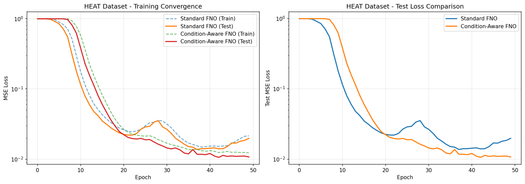
Empirical Discussion

Heat dataset. The Condition-Aware FNO achieves a lower and more stable final test loss, along with a much smoother descent. We observe jumps in the standard FNO training curve around epochs 20–30, indicating numerical instability as the ill-conditioned modes “bounce around” the narrow valleys of the loss landscape.

The smoother descent observed in the condition-aware scheme indicates a more “spherical,” isotropic loss landscape with gradients pointing more directly to the minimum. Additionally, with noisy modes filtered out, the FNO no longer fits to noise and reaches a faster convergence.

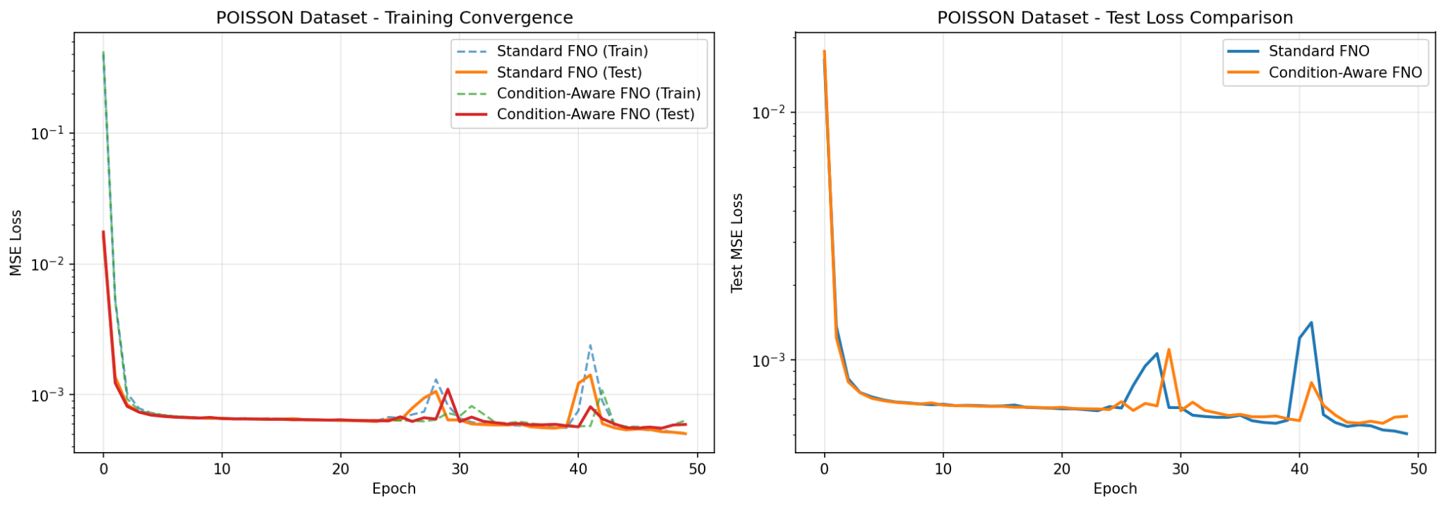
Poisson dataset. The Poisson dataset demonstrates little to no improvement in test/train loss as well as similar training curves. Since the Poisson dataset is an elliptic PDE with solutions exhibiting rapid spectral decay, the low-frequency modes contain nearly all signal information, which renders the adaptive truncation nearly meaningless.

Additionally, the “noise” in low modes in the smooth Poisson dataset is negligible — this regularization does not reduce variance, and instead introduces bias, oversmoothing the weights of valid signal modes and ultimately creating underfitting, explaining the poor performance of the condition-aware scheme.

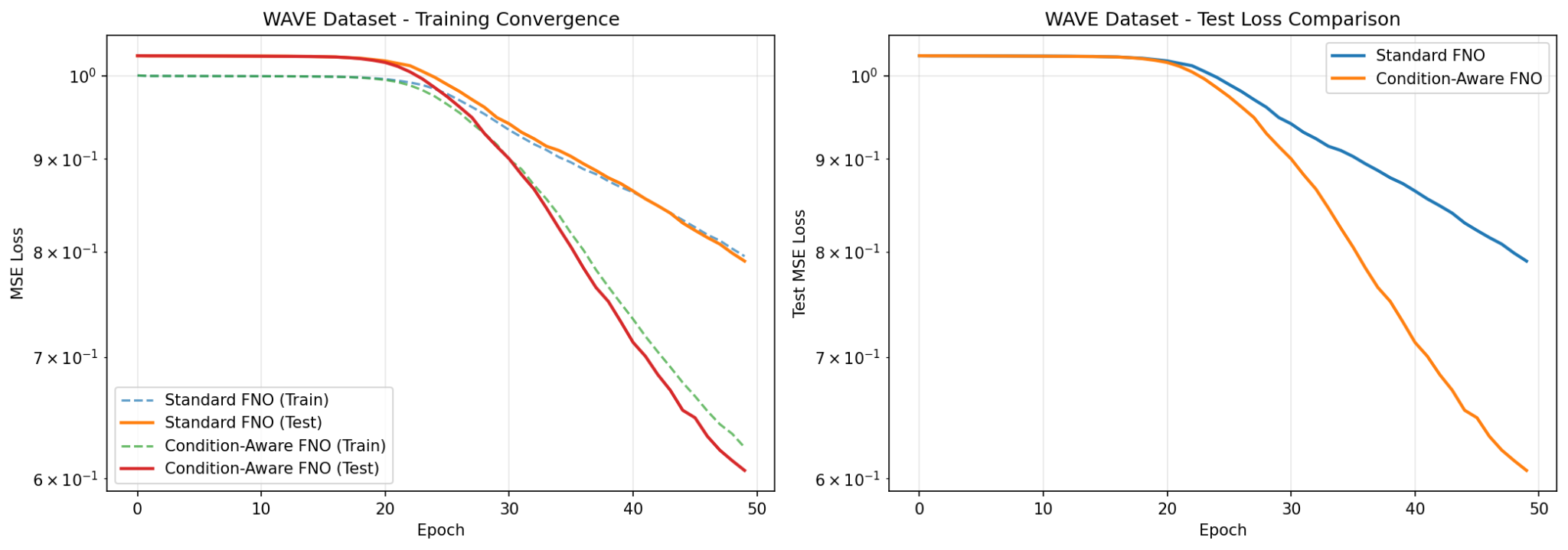
Wave dataset. In wave (hyperbolic PDE) datasets, the high-frequency features are preserved and do not smooth out initial conditions as quickly as parabolic equations. This means significant energy exists in higher frequencies, which is shown in the standard FNO’s poor performance using fixed hard truncation, discarding these physically significant high-frequency modes. The condition-aware FNO adapts the truncation boundary, retaining energy-dominant high-frequency modes that are important in wave dynamics.

Overall, we observe a significant and consistent improvement in performance in nonsmooth datasets where high-energy modes with potentially numerically unstable modes contain significant signal energy.

Gradient Descent Convergence

Hessian Spectrum and Conditioning

We recall the function for learning spectral weights $C_k$ for a specific mode $k$ with Tikhonov regularization (Ridge Regression) as defined in Eq. (1):

$$\mathcal{L}(C_k) = \|X_k C_k^H - Y_k\|_F^2 + \lambda_k \|C_k\|_F^2$$

The gradient of this function with respect to the conjugate of the weights $C_k$ is:

$$\nabla_{C_k} \mathcal{L} = (X_k^H X_k + \lambda_k I)C_k^H - X_k^H Y_k$$

The Hessian matrix $H_k$, which defines the curvature of the loss landscape, is given by the following positive definite matrix:

$$H_k = X_k^H X_k + \lambda_k I$$

Let the SVD of the data matrix $X_k$ be $U \Sigma V^H$, with singular values $\sigma_i$ for $i=1, \dots, d_{in}$. The eigenvalues of the unregularized covariance matrix $X_k^H X_k$ are $\mu_i = \sigma_i^2$. Thus, the eigenvalues of the regularized Hessian $H_k$ are:

$$\nu_i = \sigma_i^2 + \lambda_k$$

Convergence Rate of Gradient Descent

For a quadratic convex problem, Gradient Descent with an optimal step size converges linearly with a rate determined by the spectral condition number $\kappa$ of the Hessian. The error at step $t+1$ is bounded by:

$$\|\epsilon_{t+1}\| \le \left( \frac{\kappa - 1}{\kappa + 1} \right) \|\epsilon_t\|$$

We compare the condition numbers of the standard formulation ($\kappa_{\text{std}}$) and the Condition-Aware regularized formulation ($\kappa_{\text{reg}}$).

Standard FNO: For the unregularized case ($\lambda_k = 0$):

$$\kappa_{\text{std}} = \frac{\max_i(\sigma_i^2)}{\min_i(\sigma_i^2)} = \left( \frac{\sigma_{\max}}{\sigma_{\min}} \right)^2$$

High-frequency modes often exhibit rapid spectral decay, leading to $\sigma_{\min} \to 0$. This causes $\kappa_{\text{std}} \to \infty$, resulting in an “elongated” loss landscape where gradient descent converges arbitrarily slowly or oscillates.

Condition-Aware FNO: For the proposed method with $\lambda_k > 0$:

$$\kappa_{\text{reg}} = \frac{\sigma_{\max}^2 + \lambda_k}{\sigma_{\min}^2 + \lambda_k}$$

Proof. Let $a = \sigma_{\max}^2$ and $b = \sigma_{\min}^2$, with $a > b \ge 0$. We want to show $\frac{a + \lambda_k}{b + \lambda_k} < \frac{a}{b}$:

$$b(a + \lambda_k) < a(b + \lambda_k) \implies ab + b\lambda_k < ab + a\lambda_k \implies b\lambda_k < a\lambda_k$$

Since $\lambda_k > 0$, we divide by $\lambda_k$ to get $b < a$, which holds by assumption. $\square$

Conclusion

Since $\kappa_{\text{reg}} < \kappa_{\text{std}}$, the convergence factor satisfies

$$\frac{\kappa_{\text{reg}} - 1}{\kappa_{\text{reg}} + 1} < \frac{\kappa_{\text{std}} - 1}{\kappa_{\text{std}} + 1}$$

This inequality theoretically confirms the empirical results, proving that the Condition-Aware FNO operates on a better-conditioned optimization landscape. The regularization $\lambda_k$ effectively “spheres” the loss geometry, removing the narrow valleys in ill-conditioned high-frequency modes and enabling faster convergence.

Potential Methodological Extensions

Some ideas I had for extensions and fixing methodological weaknesses.

The condition-aware truncation above establishes a principled pre-training framework for mode selection, but several natural limitations motivate further development. First, a fixed $\lambda_k$ applied uniformly across modes introduces unnecessary bias on well-conditioned modes, directly explaining the degraded Poisson performance. Second, the truncation set $\mathcal{S}$ is computed once from the raw input–output pairs and never updated as the network’s internal representations evolve. Third, the spectral geometry of a deep FNO is not uniform across layers — yet a single global $\mathcal{S}$ is applied at every depth. Finally, the formulation is restricted to one-dimensional domains, whereas most physically relevant FNO benchmarks operate on 2D or 3D grids.

This section formalizes four extensions that address each of these limitations in turn.

Learnable Regularization via Bilevel Optimization

The regularization parameter $\lambda_k$ in Eq. (1) currently plays a dual role: it stabilizes ill-conditioned modes and simultaneously smooths the weights of well-conditioned ones. For smooth PDE solutions such as the Poisson dataset, the low-frequency modes are inherently stable ($\sigma_{k,\min}$ is large), so any positive $\lambda_k$ introduces avoidable bias. Conversely, for high-frequency modes in the wave dataset, a large $\lambda_k$ is genuinely necessary. A mode-adaptive, learned $\lambda_k$ would collapse to near zero for stable modes while remaining large for unstable ones.

We treat each $\lambda_k \ge 0$ as a hyperparameter optimized on a held-out validation set. Since the inner optimization problem (ridge regression) admits a closed-form solution, we can differentiate through it analytically without approximation. Formally, the bilevel problem is:

$$\min_{\boldsymbol{\alpha}} \; \mathcal{L}_{\mathrm{val}}\!\left(C_k^*(\boldsymbol{\alpha})\right) \quad \text{subject to} \quad C_k^*(\boldsymbol{\alpha}) = \operatorname*{arg\,min}_{C_k} \mathcal{L}_{\mathrm{train}}(C_k,\, e^{\alpha_k}) \tag{2}$$

where we reparameterize $\lambda_k = e^{\alpha_k}$ to enforce positivity. The inner problem has the closed-form solution

$$(C_k^*)^H = \bigl(\mathbf{X}_k^H \mathbf{X}_k + e^{\alpha_k} I\bigr)^{-1} \mathbf{X}_k^H \mathbf{Y}_k^{\mathrm{tr}}$$

and the validation loss is

$$\mathcal{L}_{\mathrm{val}}(C_k^*) = \bigl\|\mathbf{X}_k^{\mathrm{val}} (C_k^*)^H - \mathbf{Y}_k^{\mathrm{val}}\bigr\|_F^2$$

Analytic Gradient. Let $A_k = \mathbf{X}_k^H \mathbf{X}_k + e^{\alpha_k} I$. By the chain rule and the matrix inverse derivative identity $\frac{d}{d\alpha_k} A_k^{-1} = -A_k^{-1} \frac{dA_k}{d\alpha_k} A_k^{-1}$:

$$\frac{\partial \mathcal{L}_{\mathrm{val}}}{\partial \alpha_k} = \operatorname{tr}\!\left[ \frac{\partial \mathcal{L}_{\mathrm{val}}}{\partial (C_k^*)^H} \cdot \frac{\partial (C_k^*)^H}{\partial \alpha_k} \right] \tag{3}$$

where

$$\frac{\partial (C_k^*)^H}{\partial \alpha_k} = -e^{\alpha_k} A_k^{-2} \mathbf{X}_k^H \mathbf{Y}_k^{\mathrm{tr}}$$

All quantities in Eq. (3) are computable in closed form via the pre-computed SVD $\mathbf{X}_k = U_k \Sigma_k V_k^H$: the matrix inverse $A_k^{-1}$ is $V_k \operatorname{diag}(\sigma_{k,i}^2 + e^{\alpha_k})^{-1} V_k^H$, reducing the cost to $O(d_{in}^2)$ per mode after the initial SVD.

Optimization Procedure. We solve the bilevel problem with the following alternating procedure, which runs entirely before FNO training begins:

Algorithm 1: Learnable Regularization Pre-computation
Require: Training data {(X_k^tr, Y_k^tr)}_k, validation data {(X_k^val, Y_k^val)}_k,
         outer step size β, iterations T
Initialize α_k ← 0 for all k (i.e., λ_k = 1)
for t = 1, ..., T do
    for each mode k in parallel do
        Compute C_k*(α_k) via closed-form solution
        Compute ∇_{α_k} L_val via Eq. (3)
        α_k ← α_k − β ∇_{α_k} L_val
    end for
end for
return {λ_k = e^{α_k}}_k

This procedure is still a pre-computation and does not alter the FNO architecture or training loop. Its cost per iteration is $O(K \cdot d_{in}^2)$ where $K = |\mathcal{K}|$ is the number of candidate modes, and $T \sim 50$–$100$ outer iterations typically suffice.

Proof. When $\sigma_{k,i}^2 \gg e^{\alpha_k}$ for all $i$, the matrix $A_k^{-1} \approx V_k \operatorname{diag}(\sigma_{k,i}^{-2}) V_k^H = (\mathbf{X}_k^H \mathbf{X}_k)^{-1}$, the ordinary least-squares inverse. Hence $C_k^* \to C_k^{\mathrm{OLS}}$ and $\mathcal{L}_{\mathrm{val}}$ is insensitive to further changes in $\alpha_k$, driving $\nabla_{\alpha_k} \mathcal{L}_{\mathrm{val}} \to 0$. $\square$

Per-Layer Spectral Truncation

The current framework scores modes using the raw input–output data pairs $(v, u)$ and applies the resulting set $\mathcal{S}$ uniformly at every FNO layer $\ell = 1, \dots, L$. However, the feature field $v_\ell(x)$ undergoes substantial transformation with depth: early layers tend to retain input-like spectral content, while later layers increasingly encode solution-like representations. A single global $\mathcal{S}$ cannot simultaneously reflect the spectral geometry of all layers.

We define a separate truncation set $\mathcal{S}^\ell \subseteq \mathcal{K}$ for each layer $\ell$, constructed from the layer’s actual intermediate representations. Because these representations depend on the trained network weights, we adopt a two-pass bootstrap procedure.

Definition 4.2 (Layer-$\ell$ Data Matrices). Given a trained FNO with feature fields $\{v_\ell^{(s)}\}_{s=1}^N$ extracted at layer $\ell$ on the training set, define

$$\mathbf{X}_k^\ell = \begin{bmatrix} \hat{v}_\ell^{(1)}(k)^H \\ \vdots \\ \hat{v}_\ell^{(N)}(k)^H \end{bmatrix} \in \mathbb{C}^{N \times w_\ell}, \quad \mathbf{Y}_k^\ell = \begin{bmatrix} \hat{v}_{\ell+1}^{(1)}(k)^H \\ \vdots \\ \hat{v}_{\ell+1}^{(N)}(k)^H \end{bmatrix} \in \mathbb{C}^{N \times w_{\ell+1}}$$

where $w_\ell$ denotes the channel width at layer $\ell$.

The per-layer utility score is computed identically:

$$\mathrm{score}^\ell(k) = \frac{\|\mathbf{Y}_k^\ell\|_F^2}{\kappa(\mathbf{X}_k^\ell)}$$

Algorithm 2: Bootstrap Per-Layer Truncation
Require: Training data, energy threshold η, bootstrap epochs T_0
Train a baseline CA-FNO with global S for T_0 epochs
for each layer ℓ = 1, ..., L do
    Forward-pass training set; extract {v_ℓ^(s)} and {v_{ℓ+1}^(s)}
    Compute X_k^ℓ, Y_k^ℓ, SVD, and score^ℓ(k) for all k
    Construct S^ℓ via energy criterion
end for
Retrain FNO from scratch using {S^ℓ}_{ℓ=1}^L

The bootstrap run need not be trained to full convergence; $T_0 \approx 10$–$20\%$ of total training epochs is sufficient to obtain representative intermediate representations for scoring.

Conversely, for a hyperbolic PDE (e.g., wave equation), energy is conserved across frequencies and the inclusion may not hold, motivating empirical verification via Algorithm 2.

Dynamic Spectral Truncation

Both the global and per-layer truncation schemes commit to a fixed mode set before or at the beginning of training. During training, the network’s predictions improve, and the residual between predictions and targets — not the original output $u$ — characterizes what information remains to be learned. Modes that appeared noise-dominated relative to the raw output may carry structured residual signal at later epochs. Dynamic truncation re-evaluates $\mathcal{S}$ periodically against the current residuals.

Let $\hat{u}_\theta^{(s)}(x)$ denote the network’s prediction at training epoch $t$, and define the residual at each training sample as

$$r^{(s)}(x) = u^{(s)}(x) - \hat{u}_\theta^{(s)}(x)$$

The residual Fourier coefficients are $\hat{r}^{(s)}(k) = \mathcal{F}[r^{(s)}](k)$. We construct residual target matrices

$$\mathbf{R}_k^{(t)} = \begin{bmatrix} \hat{r}^{(1)}(k)^H \\ \vdots \\ \hat{r}^{(N)}(k)^H \end{bmatrix} \in \mathbb{C}^{N \times d_{out}}$$

and re-score each mode using the residual energy:

$$\mathrm{score}_t(k) = \frac{\|\mathbf{R}_k^{(t)}\|_F^2}{\kappa(\mathbf{X}_k)} \tag{4}$$

where $\mathbf{X}_k$ (derived from inputs $v^{(s)}$) is fixed across re-evaluations since the inputs do not change. Only $\mathbf{R}_k^{(t)}$ is updated.

Let $\mathcal{T} = \{t_1, t_2, \dots, t_m\}$ be a sequence of re-evaluation epochs. At each $t_i \in \mathcal{T}$, we recompute $\mathbf{R}_k^{(t_i)}$ and update $\mathcal{S}$. Modes are added or dropped from the active set accordingly, and the FNO’s spectral multiplier matrices $M_\ell(k)$ for newly excluded modes are zeroed out.

A geometric schedule $t_i = \lfloor t_{\max} \cdot \rho^{m-i} \rfloor$ for $\rho \in (0,1)$ concentrates re-evaluations toward the end of training, where residual structure is most informative. In practice, $m = 3$–$5$ re-evaluations suffice.

Re-evaluations $m$	Heat Test Loss	Wave Test Loss
0 (static)	baseline	baseline
1	$-\delta_1$	$-\delta_1'$
3	$-\delta_3$	$-\delta_3'$
5	$-\delta_5$	$-\delta_5'$

This implies that dynamic truncation will tend to drop modes over time for parabolic PDEs as the network learns to explain their contribution, progressively shrinking $\mathcal{S}^{(t)}$. For hyperbolic PDEs, dynamic re-evaluation allows previously excluded high-frequency modes to be activated if the residual reveals unlearned structure.

Re-scoring requires recomputing $\mathbf{R}_k^{(t)}$ for all modes $k$, which costs one forward pass over the training set plus $O(K \cdot N \cdot d_{out})$ to compute the Frobenius norms. Since $\mathbf{X}_k$ is fixed, no additional SVD computations are required.

Extension to Two-Dimensional Domains

The foregoing development assumes a one-dimensional spatial domain, yielding scalar wavenumbers $k \in \mathbb{Z}$. In practice, the most widely studied FNO benchmarks — two-dimensional Darcy flow and the vorticity formulation of Navier-Stokes — operate on two-dimensional grids of resolution $N_1 \times N_2$. Extending to 2D introduces both additional notation and a nontrivial geometric question: whereas standard FNO in 2D uses a rectangular truncation in frequency space, the condition-aware criterion may select an irregular subset $\mathcal{S} \subseteq \mathbb{Z}^2$, providing new information about the anisotropic spectral structure of the underlying PDE.

Let the domain be $D = [0,1]^2$ discretized at resolution $N_1 \times N_2$. Modes are indexed by 2D wavenumber pairs $\mathbf{k} = (k_1, k_2) \in \mathcal{K}^{2D} \subseteq \mathbb{Z}^2$. The 2D DFT of the input and output functions are

$$\hat{v}(\mathbf{k}) = \mathcal{F}_{2D}[v](\mathbf{k}) \in \mathbb{C}^{d_{in}}, \quad \hat{u}(\mathbf{k}) = \mathcal{F}_{2D}[u](\mathbf{k}) \in \mathbb{C}^{d_{out}}$$

The data matrices are constructed per 2D mode identically to the 1D case, and the utility score and energy criterion extend without modification:

$$\mathrm{score}(\mathbf{k}) = \frac{\|\mathbf{Y}_\mathbf{k}\|_F^2}{\kappa(\mathbf{X}_\mathbf{k})}, \quad \mathcal{S}^{2D} = \operatorname*{arg\,min}_{S \subseteq \mathcal{K}^{2D}} |S| \quad \text{s.t.} \quad \sum_{\mathbf{k} \in S} \mathrm{Energy}(\mathbf{k}) \ge \eta \sum_{\text{all } \mathbf{k}} \mathrm{Energy}(\mathbf{k}) \tag{5}$$

Anisotropic Spectral Geometry. Unlike the 1D case, the selected set $\mathcal{S}^{2D}$ need not be a square or rectangular region in $\mathbb{Z}^2$. The shape of $\mathcal{S}^{2D}$ is physically informative:

• For isotropic PDEs (e.g., 2D heat equation, isotropic Darcy flow), the energy depends only on $|\mathbf{k}| = \sqrt{k_1^2 + k_2^2}$, and $\mathcal{S}^{2D}$ will approximate a disk of radius $K^*$ in frequency space.
• For problems with directional features (e.g., shear flows, anisotropic diffusion), $\mathrm{Energy}(\mathbf{k})$ will be elongated along one axis, and $\mathcal{S}^{2D}$ will reflect this asymmetry — modes along the dominant direction will be retained to higher wavenumbers than modes in the orthogonal direction.

This geometric structure directly encodes the anisotropy of the physical system in the FNO architecture and cannot be recovered by any rectangular truncation.

The total number of modes to score grows as $O(N_1 N_2)$ rather than $O(N_1)$, but since each mode’s SVD and scoring is independent, the computation parallelizes identically to the 1D case. The SVD cost per mode remains $O(N d_{in}^2)$, so the total pre-computation cost is $O(N_1 N_2 \cdot N \cdot d_{in}^2)$, which for typical FNO resolutions ($N_1 = N_2 = 64$, $N = 1000$, $d_{in} = 1$) is on the order of $4 \times 10^6$ operations.

In the isotropic case, Eq. (5) recovers a radial spectral truncation $\mathcal{S}^{2D} \approx \{\mathbf{k} : |\mathbf{k}| \le K^*\}$ for some data-driven $K^*$, providing a theoretical connection to classical spectral methods in which cutoff wavenumbers are chosen based on the Kolmogorov microscale or solution regularity.

References

[1] Zongyi Li, Nikola B. Kovachki, Kamyar Azizzadenesheli, Burigede Liu, Kaushik Bhattacharya, Andrew M. Stuart, and Anima Anandkumar. Fourier neural operator for parametric partial differential equations. CoRR, abs/2010.08895, 2020.