dvd km

Visualization code for this post: github.com/dvdawg/qnl-prep

Note: throughout this post, we often omit a factor of $\hbar$ in Hamiltonians. This is done to work with frequencies rather than energies — recall that the units of $\hbar$ are $\text{J}\cdot\text{s}$.

Two-Level System

Finding the time-dependent wavefunction

For Hamiltonian $\hat{H} = \omega\hat{\sigma}_z$, we use the time evolution unitary $\hat{U} = e^{-i\hat{H}t/\hbar}$ to transform our initial state $\ket{\psi} = \alpha\ket{0}+\beta\ket{1}$. Recall that the unitary transformation of any generator operator $\hat{G}$ is

$$\hat{U}=e^{-i\hat{G}t/\hbar}$$

Using the Hamiltonian in this expression creates a phase for both $\ket{0}$ and $\ket{1}$, introducing time evolution as the transformation to our wavefunction. We evaluate the behavior of the Hamiltonian when applied to the basis:

$$\hat{H}\ket{0} = \omega\ket{0} \;\implies\; e^{-i\hat{H}t/\hbar}=e^{-i\omega t/\hbar}$$ $$\hat{H}\ket{1} = -\omega\ket{1}\;\implies\; e^{-i\hat{H}t/\hbar}=e^{i\omega t/\hbar}$$

and thus gives the following expression when inserted into our original state:

$$\ket{\psi(t)} = \alpha e^{-i\omega t/\hbar}\ket{0} + \beta e^{i\omega t/\hbar}\ket{1}$$

The Bloch Sphere

We can prove any generic state $\ket{\psi}$, up to a global phase, is mappable to a point on the surface of a sphere. Starting from $\ket{\psi} = \alpha e^{i\omega_1 t/\hbar}\ket{0} + \beta e^{i\omega_2 t/\hbar}\ket{1}$, since only the relative phase has physical meaning, we rewrite as

$$\ket{\psi}=\alpha\ket{0} + \beta e^{i(\omega_2-\omega_1)t/\hbar}\ket{1}$$

Using $\alpha^2+\beta^2=1$, we reparameterize into the form

$$\ket{\psi(t)} = \cos\frac{\theta}{2}\ket{0} + \sin\frac{\theta}{2}e^{i\phi}\ket{1}, \quad \theta \in[0, \pi], \ \phi\in[0, 2\pi)$$

With this parameterization, we can use $\theta, \phi$ as spherical coordinates with radius 1 to define points on the unit sphere. In Cartesian coordinates:

$$\vec{r}=\sin\theta\cos\phi\ \hat{x}\ + \sin\theta\sin\phi\ \hat{y}\ + \cos\theta\ \hat{z}$$

Defining $\alpha'=\alpha e^{i\omega_1 t/\hbar}$ and $\beta'=\beta e^{i\omega_1 t/\hbar}$, we can re-express the Cartesian vector as:

$$\vec{r} = 2\operatorname{Re}(\alpha'^*\beta')\ \hat{x}+2\operatorname{Im}(\alpha'^*\beta')\ \hat{y}+(\alpha'^2-\beta'^2)\hat{z}$$

Alternative representation via density matrix. The density matrix of this pure state is

$$\rho=\frac{1}{2}\begin{pmatrix}1+\cos\theta& e^{-i\phi}\sin\theta \\ e^{-i\phi}\sin\theta & 1+\sin\theta\end{pmatrix}=\begin{pmatrix}|\alpha'|^2 & \alpha'\beta'^*\\\alpha'^*\beta' &|\beta'|^2\end{pmatrix}$$

The $x, y, z$ coordinates correspond to expectation values of the Pauli matrices,

$$x = \bra{\psi}\hat{\sigma}_x\ket{\psi}, \quad y=\bra{\psi}\hat{\sigma}_y\ket{\psi}, \quad z=\bra{\psi}\hat{\sigma}_z\ket{\psi}$$

which follows from $\bra{\psi}\hat{\sigma}_i\ket{\psi}=\mathrm{Tr}(\rho\sigma_i)$:

$$\bra{\psi}\hat{\sigma}_i\ket{\psi}=\mathrm{Tr}\ (\rho\sigma_i)=\frac{1}{2}\left(x\ \mathrm{Tr}\ (\sigma_x\sigma_i)+y\ \mathrm{Tr}\ (\sigma_y\sigma_i)+z\ \mathrm{Tr}\ (\sigma_z\sigma_i)\right)=r_i$$

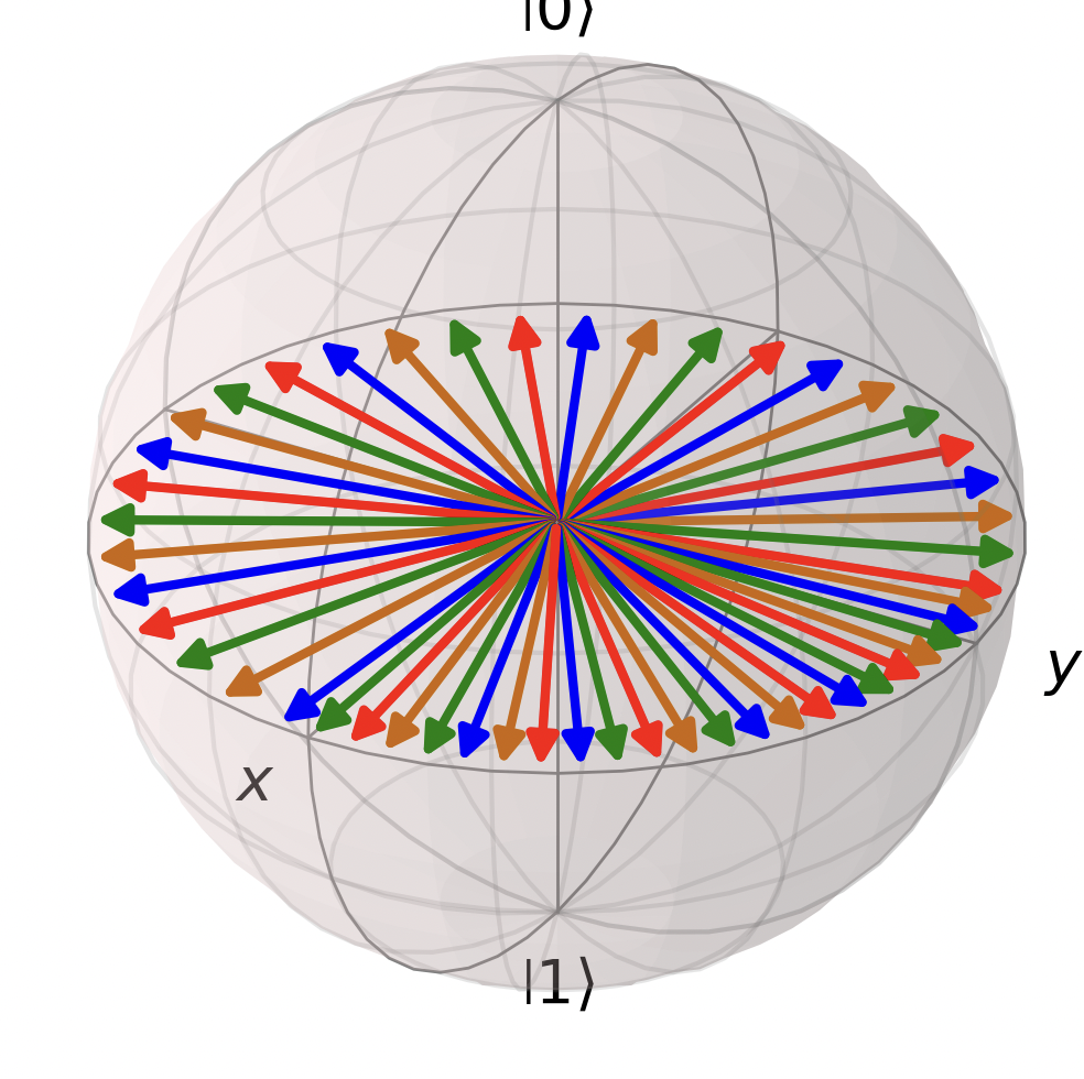
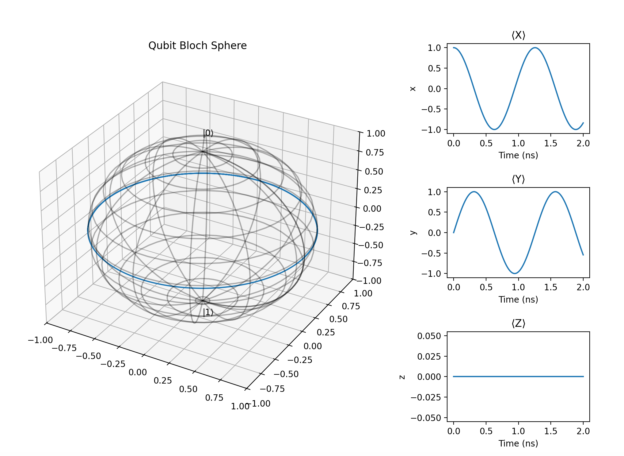
Bloch sphere visualizations with initial conditions $\alpha=\frac{1}{\sqrt{2}}, \beta=\frac{1}{\sqrt{2}}$, created with qutip and matplotlib:

Driving Field

Mathematical Derivation with Rotating-Wave Approximation

We now consider the Hamiltonian $\hat{H} = \frac{\omega_q\hat{\sigma}_z}{2} + A\cos(\omega_d t + \phi) \hat{\sigma}_x$, focusing first on the resonant case $\omega_q=\omega_d$.

We shift into the rotating frame via a unitary transformation

$$\hat{H}\longrightarrow\breve{H} = \hat{U}\hat{H}\hat{U}^\dag + i\hbar\dot{U}\hat{U}^\dagger$$

Defining $\Omega=Ae^{i\phi}$, the driving term becomes

$$A\cos(\omega_d t + \phi)=\frac{1}{2}\Omega e^{i\omega_dt}+\frac{1}{2}\Omega^* e^{-i\omega_dt}$$

We choose the rotation unitary based on the free Hamiltonian,

$$\hat{U} = e^{\frac{i\omega_dt}{2}\hat{\sigma}_z}=e^{-i\omega_dt/2}\ket{0}\bra{0}+e^{i\omega_dt/2}\ket{1}\bra{1}$$

Using the raising and lowering operators $\hat{\sigma}_+=\ket{0}\bra{1}$, $\hat{\sigma}_-=\ket{1}\bra{0}$ and the substitution $\hat{\sigma}_x=\hat{\sigma}_++\hat{\sigma}_-$, we find

$$e^{\frac{i\omega_dt}{2}\hat{\sigma}_z}\hat{\sigma}_xe^{-\frac{i\omega_dt}{2}\hat{\sigma}_z}=e^{i\omega_dt}\hat{\sigma}_+ +e^{-i\omega_dt}\hat{\sigma}_-$$

Expanding, setting $\omega_q=\omega_d$, and applying the rotating wave approximation (dropping terms oscillating at $2\omega_d$):

$$\hat{U}\hat{H}\hat{U}^\dag=\frac{\omega_q\hat{\sigma}_z}{2}+\frac{1}{2}(\Omega\hat{\sigma}_++\Omega^*\hat{\sigma}_-)$$

The second term of the transformation evaluates to

$$i\hbar\dot{U}\hat{U}^\dagger=-\hbar\frac{\omega_d\hat{\sigma}_z}{2}$$

Putting both terms together and canceling the $\hat{\sigma}_z$ terms with $\omega_q=\omega_d$:

$$\breve{H}=\frac{1}{2}(\Omega\hat{\sigma}_++\Omega^*\hat{\sigma}_-)=\frac{1}{2}\begin{pmatrix}0 & \Omega \\ \Omega^* & 0\end{pmatrix}$$

Visualization and Analysis

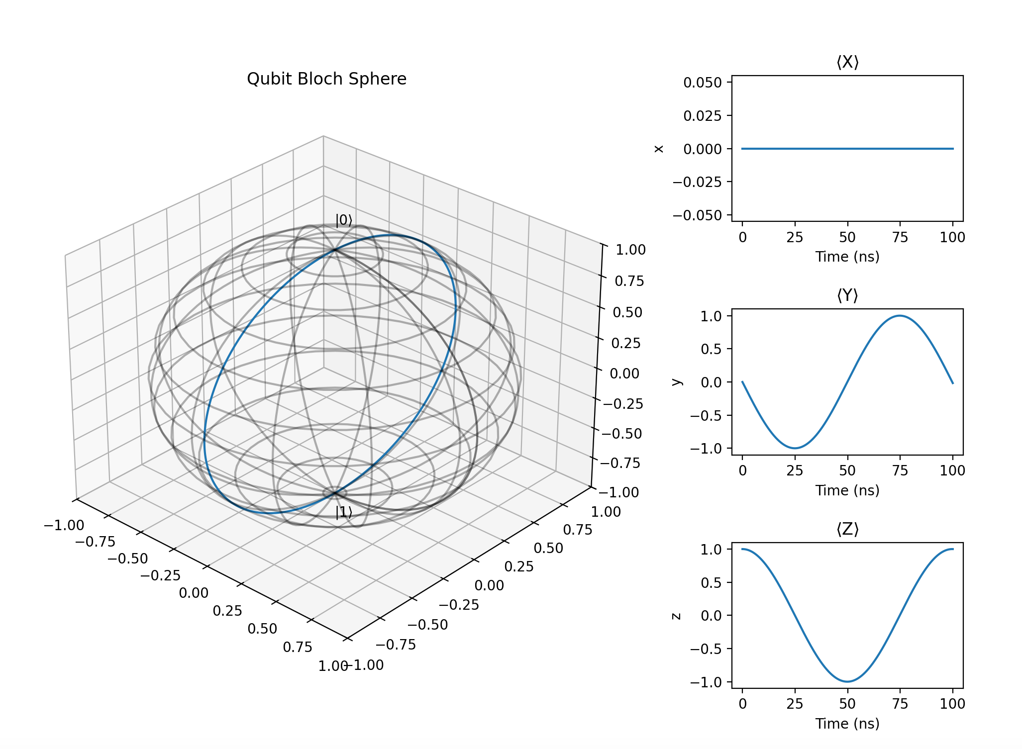
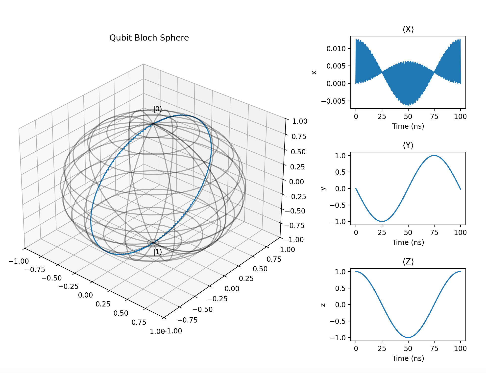
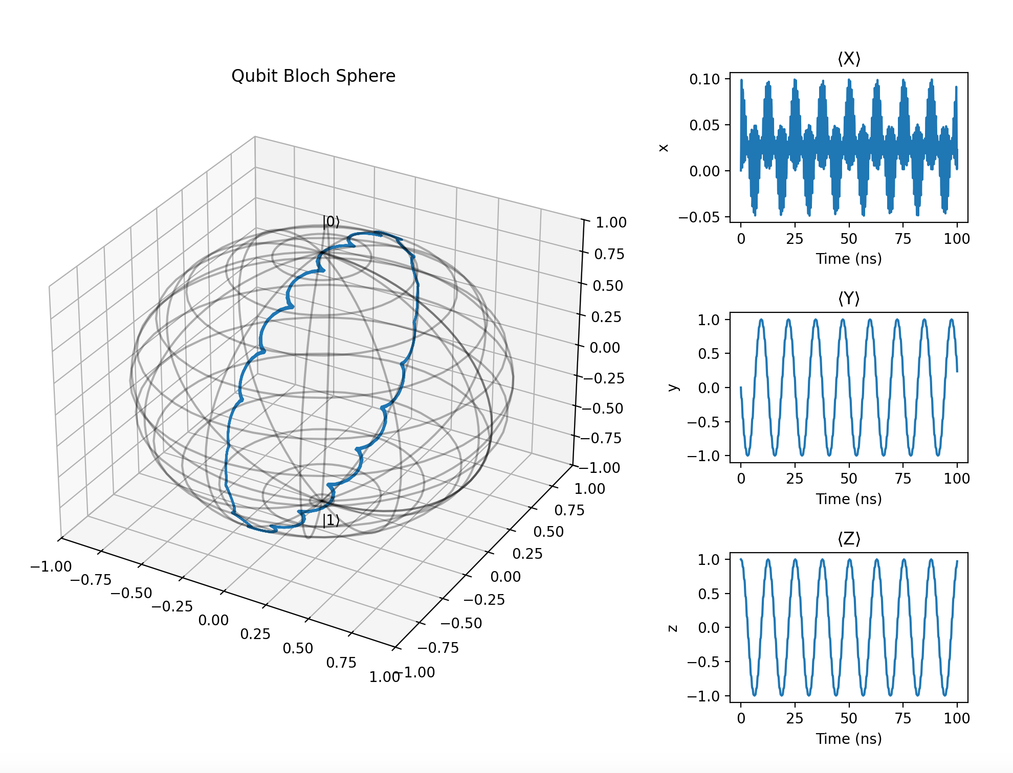
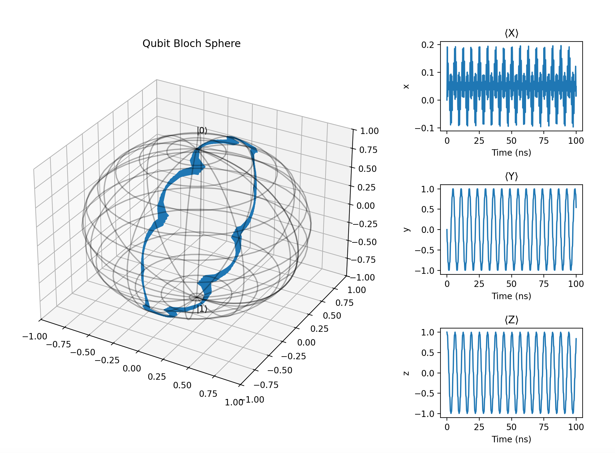
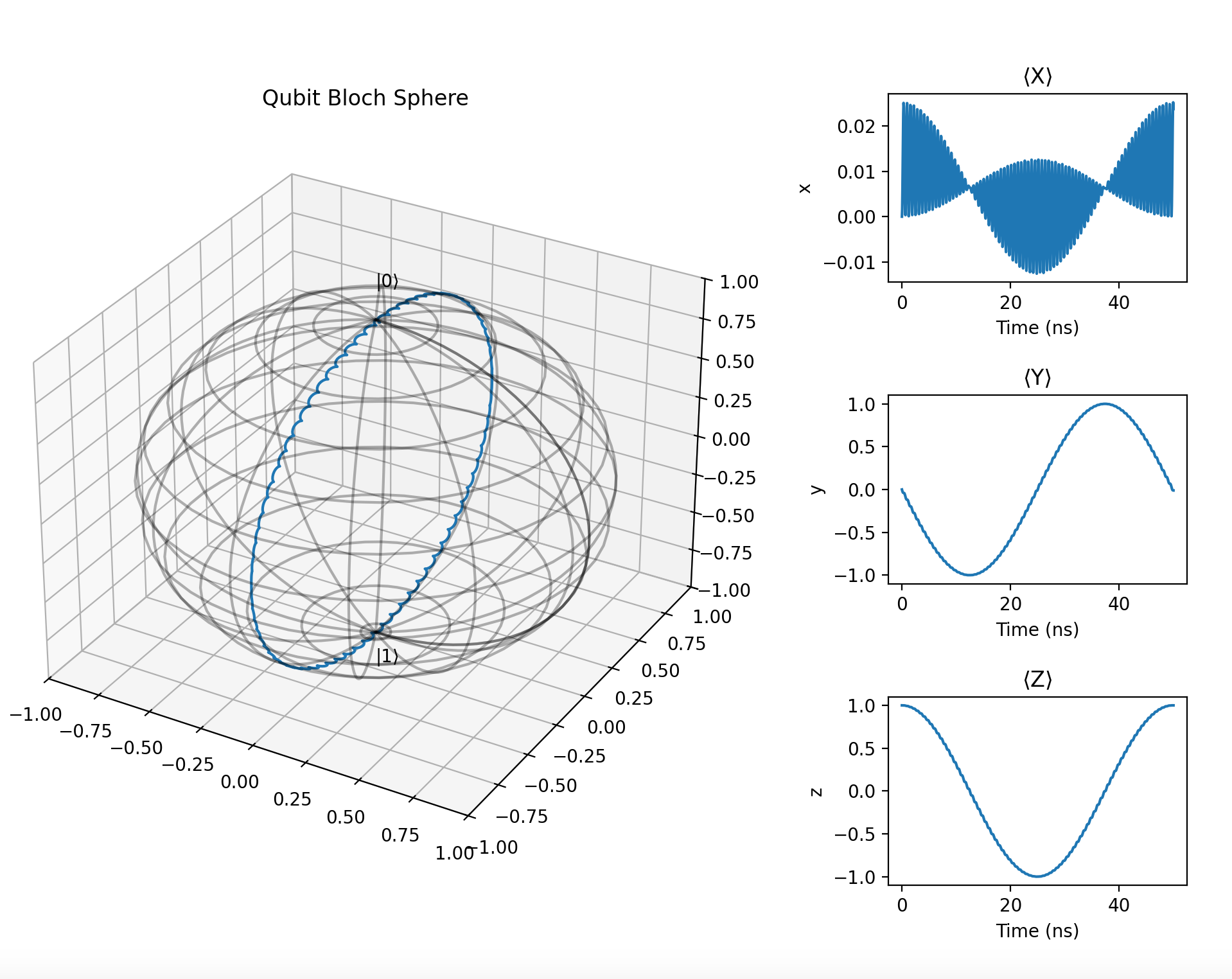
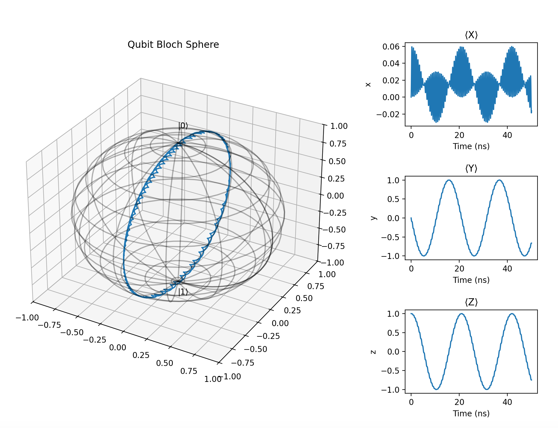
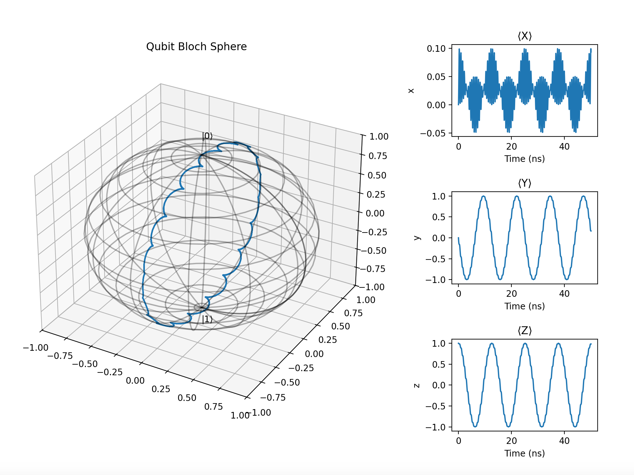
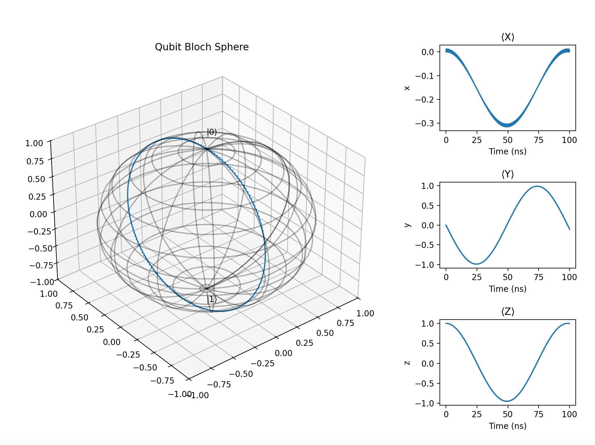
At $\omega_d = \omega_q=5.0\text{ GHz}$, we vary $A$ relative to the timescale $t$ to assess the limits of the RWA. All frequencies are in GHz, all times in ns. The initial state is $\ket{\psi_0}=\ket{0}$.

The resonant RWA baseline:

Varying $A$ at timescale $t=100\text{ ns}$:

$A=0.063,\ A/\omega_q=0.0126$

$A=0.5,\ A/\omega_q=0.1$

$A=1.0,\ A/\omega_q=0.2$

Varying $A$ at timescale $t=50\text{ ns}$:

$A=0.126,\ A/\omega_q=0.0252$

$A=0.3,\ A/\omega_q=0.06$

$A=0.5,\ A/\omega_q=0.1$

From these plots and mathematical analysis, we draw two conclusions:

1. To complete a full cycle, $A\cdot t\approx2\pi$. This gives a period of $t=\frac{2\pi}{A}$.
2. For the RWA to be valid, $A\ll\omega_q$. As a general rule, $A/\omega_q \lesssim 0.05$ yields a good approximation.

Off-Resonant Driving

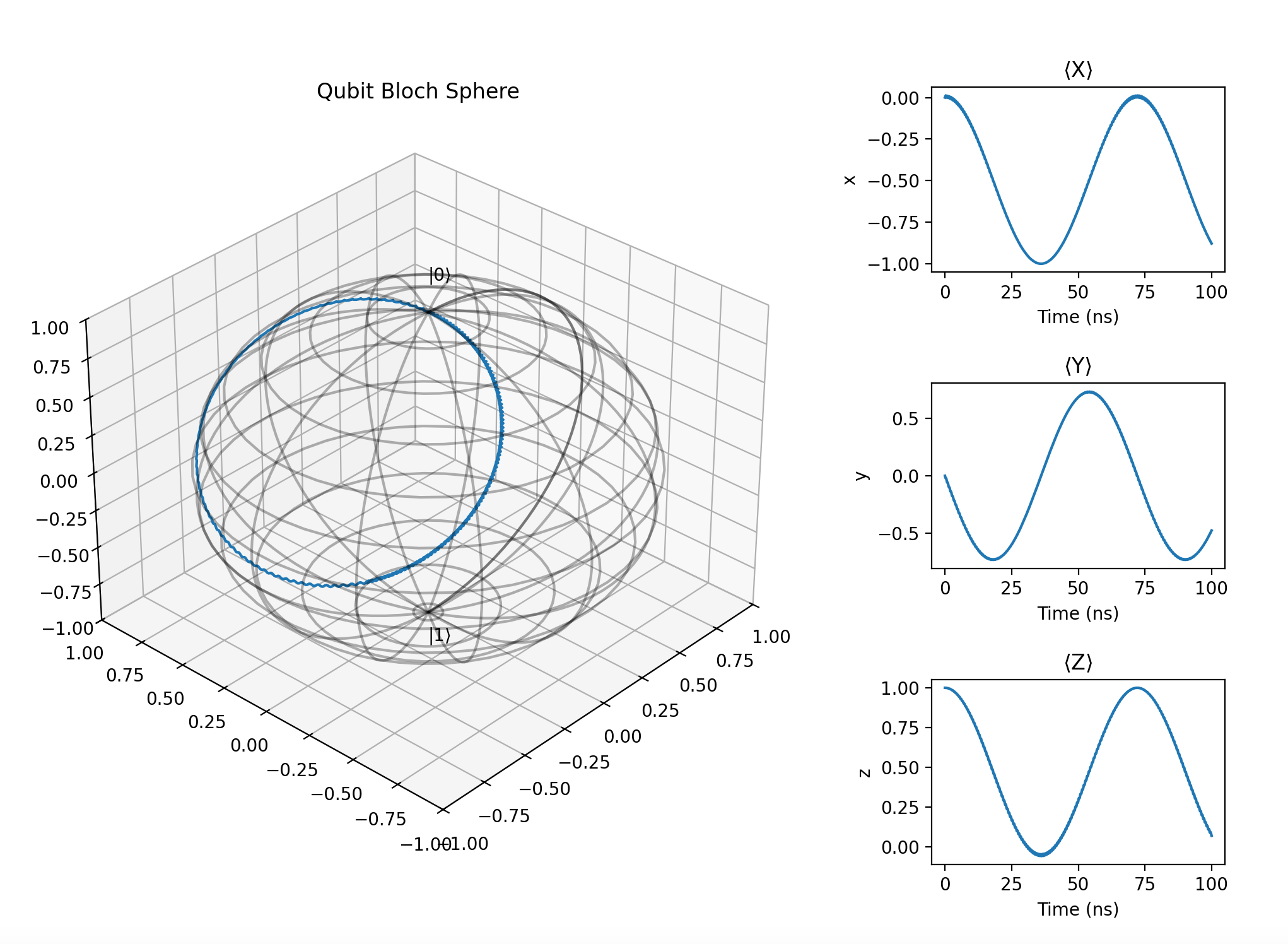
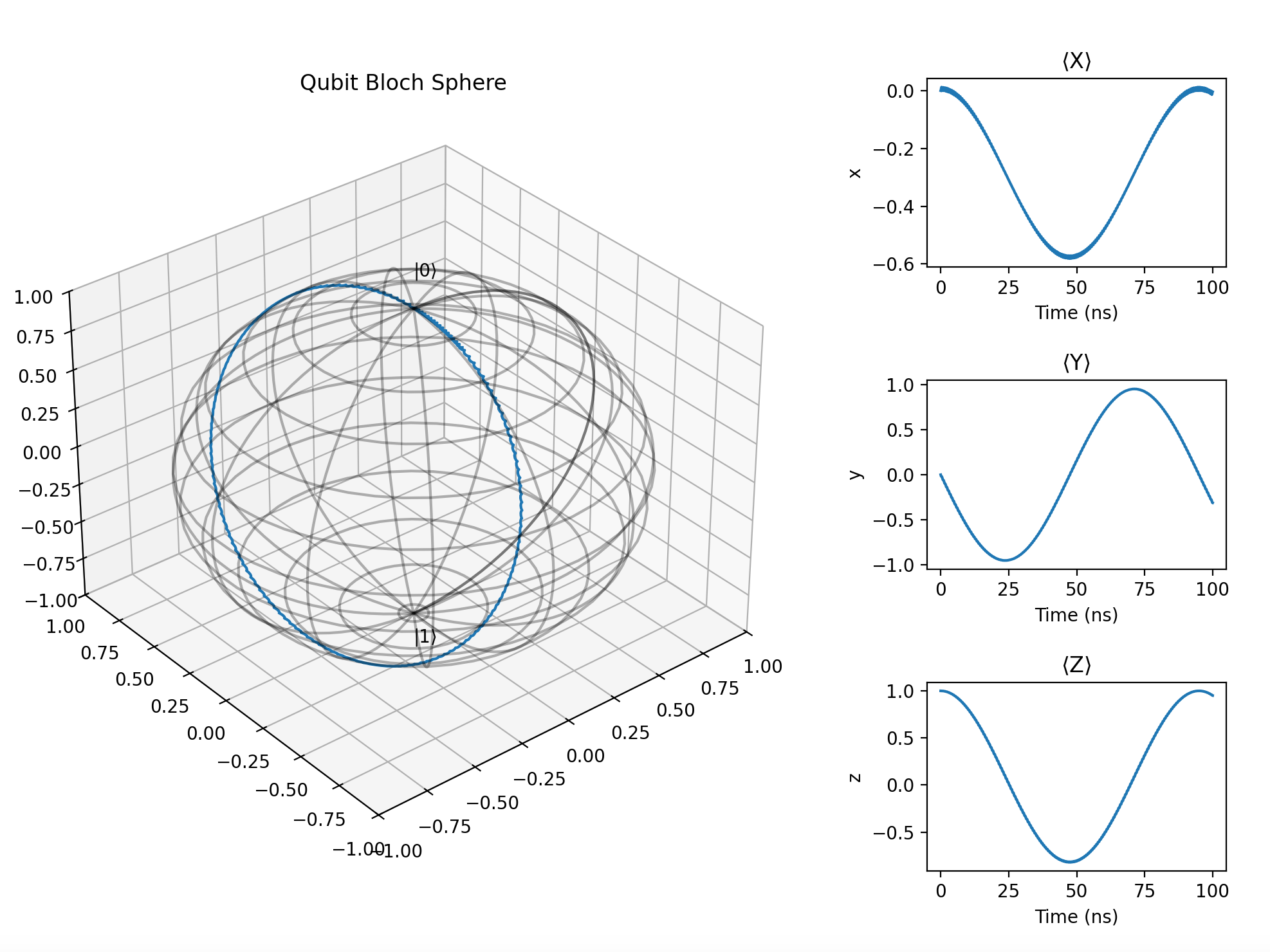
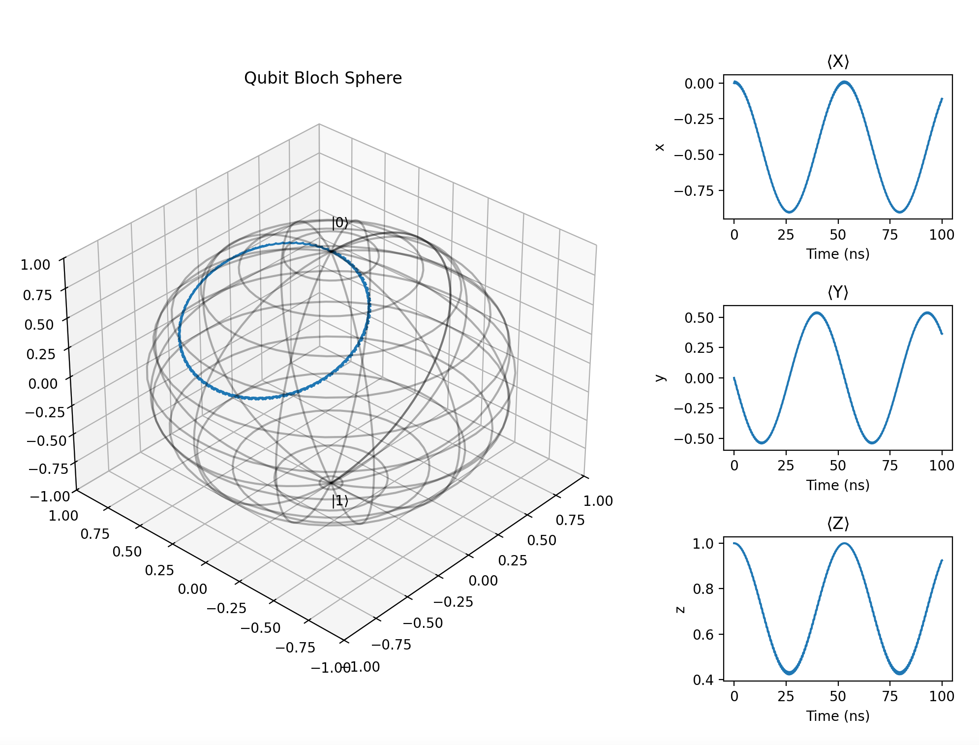
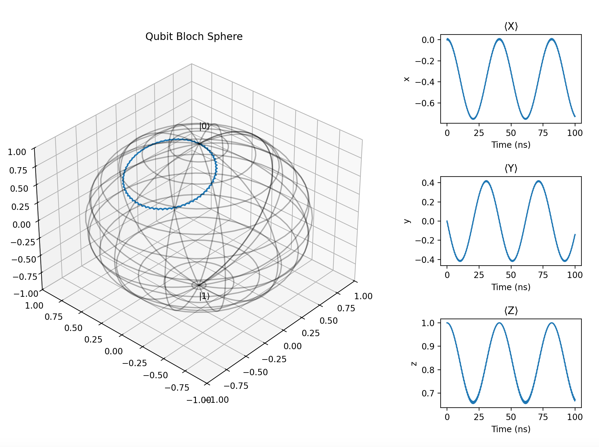
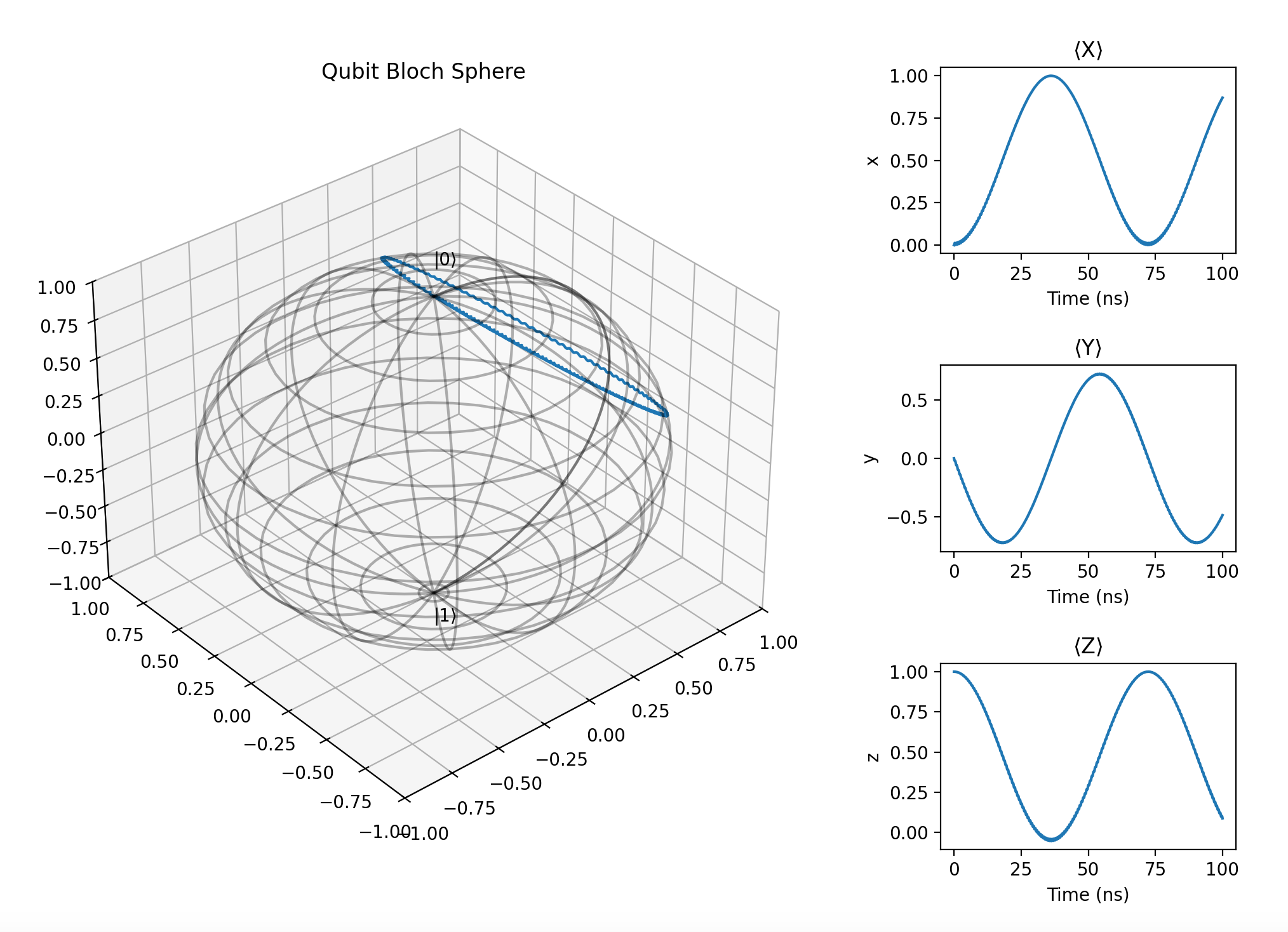
We now consider $\omega_d\neq\omega_q$ and display the effects of an off-resonant driving field. Using $\ket{\psi_0}=\ket{0}$, $t=100\text{ ns}$, $A=0.063$, and $\omega_q=5.0\text{ GHz}$:

$\omega_d=5.005$

$\omega_d=5.01$

$\omega_d=5.03$

$\omega_d=5.05$

$\omega_d=5.07$

$\omega_d=4.97$

Off-resonant driving shrinks the rotation progressively toward the initial state $\ket{0}$. As the drive frequency moves farther from the qubit frequency, the $\langle z\rangle$ plot approaches $1.00$ and the $\langle y\rangle$ plot approaches $0.00$.